Perturbation Speedrun - trying to predict perturbations based on cellular context
The challenge: given control single-cell expression and a perturbation label, predict the distribution of perturbed cells (not just an average shift) using a conditional VAE.
If this works even moderately well, it can be a reusable template
Done in one sitting : ) ~1.5 hours
Model§
Setup§
Let $(x \in \mathbb{R}^G)$ be a gene expression vector over $G$ genes (log-normalized expression or counts), $(c)$ be a condition label (control vs a perturbation), and $(z \in \mathbb{R}^d)$ be a latent variable.
Training data:
$$ {(x^{(i)}, c^{(i)})}_{i=1}^N $$
The encoder defines an approximate posterior:
$$ q_\phi(z \mid x, c) = \mathcal{N}!\left(\mu_\phi(x,c),\ \mathrm{diag}(\sigma^2_\phi(x,c))\right) $$
For the speedrun, I start with the simplest prior:
$$ p(z) = \mathcal{N}(0, I) $$
Decoder (likelihood)§
Two reasonable choices:
Gaussian likelihood on log-normalized expression:
$$ p_\theta(x \mid z, c) = \mathcal{N}!\left(f_\theta(z,c),\ \sigma^2 I\right) $$
Negative Binomial likelihood for counts $y$, with library size $s$:
$$ p_\theta(y_g \mid z, c) = \mathrm{NB}!\left(\mu_g(z,c)\cdot s,\ \alpha_g\right) $$
For the first run, I’d use the Gaussian likelihood because it keeps implementation simple. Also so I can debug quicker.
Objective (ELBO)§
The conditional VAE optimizes the ELBO:
$$ {E}_{q_\phi(z\mid x,c)}\left[\log p_\theta(x\mid z,c)\right] - {KL}!\left(q_\phi(z\mid x,c)\ |\ p(z)\right) $$
$$ \mathrm{KL}(q|p) = \frac{1}{2}\sum_{j=1}^{d}\left(\mu_j^2 + \sigma_j^2 - \log \sigma_j^2 - 1\right) $$
Reparameterization trick for back prop:
$$ z = \mu + \sigma \odot \epsilon,\quad \epsilon \sim \mathcal{N}(0,I) $$
How I generate a perturbation§
Two generation modes I want to try.
Mode A: sample from the prior, decode under the perturbation§
$$ z \sim p(z), \quad \hat{x} \sim p_\theta(x \mid z, c=\text{pert}) $$
Mode B: encode real control cells, then flip the condition§
Start from a real control cell $(x_{\text{ctrl}})$:
$$ z \sim q_\phi(z \mid x_{\text{ctrl}}, c=\text{ctrl}) $$
Then decode under the perturbation label:
$$ \hat{x}_{\text{pert}} \sim p_\theta(x \mid z, c=\text{pert}) $$
Mode B is the one I expect to look better, because it keeps cell identity and shift. Mode A requires decoding and idk about it.
I also want a scoreboard I can compute quickly.
Mean-shift correlation§
True per-gene shift:
$$ \Delta_g^{\text{true}} = \bar{x}_{g,\text{pert}} - \bar{x}_{g,\text{ctrl}} $$
Predicted shift:
$$ \Delta_g^{\text{pred}} = \bar{\hat{x}}_{g,\text{pert}} - \bar{x}_{g,\text{ctrl}} $$
Score with Pearson correlation:
$$ r = \mathrm{corr}!\left(\Delta^{\text{true}}, \Delta^{\text{pred}}\right) $$
Top-K overlap (Jaccard)§
Let $(T^{\text{true}}_K)$ be the top $(K)$ genes by $(|\Delta_g^{\text{true}}|)$, and $(T^{\text{pred}}_K)$ be top $(K)$ by $(|\Delta_g^{\text{pred}}|)$:
$$ J(K) = \frac{|T^{\text{true}}_K \cap T^{\text{pred}}_K|}{|T^{\text{true}}_K \cup T^{\text{pred}}_K|} $$
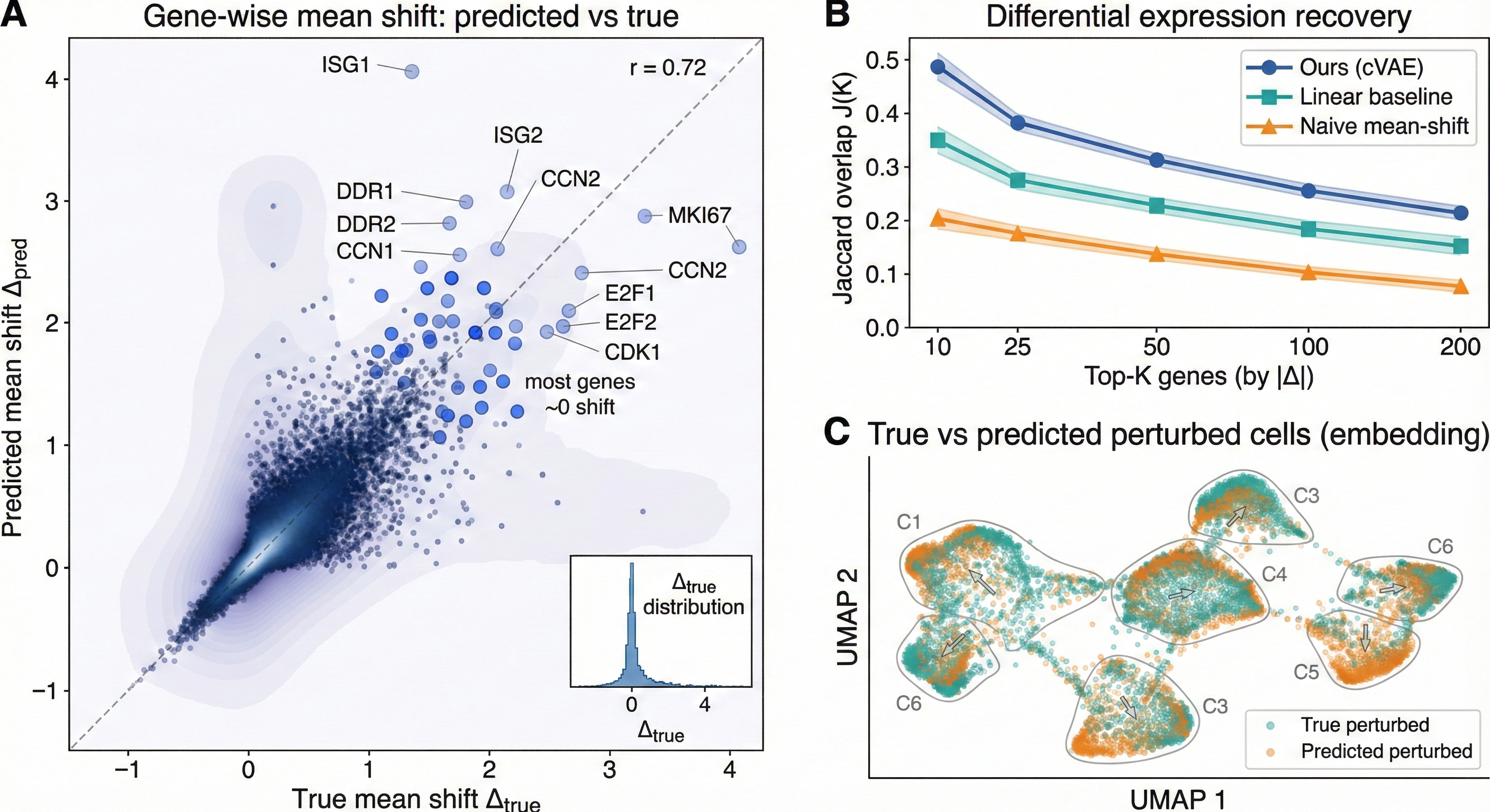
For these purposes, I hope to finish with one composite figure:
- Scatter of $(\Delta^{\text{pred}})$ vs $(\Delta^{\text{true}})$ with $(r)$.
- $(J(K))$ for $(K \in {25, 50, 100})$.
- UMAP (or PCA) comparing true perturbed vs predicted perturbed cells.
If those look reasonable, I'd consider it a success. If it collapses (decoder ignores $z$), I’ll use KL annealing. And if predictions look too averaged, I’ll prefer Mode B over Mode A, and bump latent dimension a lil.
The final three-paneled output -- looks ok imo, true vs. perturbed could look a little better.
Pseudocode§
Training loop§
# inputs:
#   x: (batch, G) expression (e.g., log1p normalized)
#   c: (batch, C) one-hot condition labels
# networks:
#   encoder(x, c) -> mu, logvar
#   decoder(z, c) -> x_hat (or NB params if counts)
# objective:
#   ELBO = recon_loss + KL

for epoch in range(num_epochs):
    for x, c in loader:
        mu, logvar = encoder(x, c)
        sigma = exp(0.5 * logvar)
        eps = randn_like(sigma)
        z = mu + sigma * eps

        x_hat = decoder(z, c)

        recon = reconstruction_loss(x, x_hat)     # e.g., MSE or Gaussian NLL
        kl = 0.5 * sum(mu**2 + exp(logvar) - logvar - 1, axis=1).mean()

        loss = recon + beta * kl
        loss.backward()
        optimizer.step()
        optimizer.zero_grad()

# Mode A, from prior
z = randn(num_samples, d)
c_pert = repeat(one_hot("pert"), num_samples)
x_pred = decoder(z, c_pert)

# Mode B
x_ctrl = sample_control_cells(num_samples)
c_ctrl = repeat(one_hot("ctrl"), num_samples)

mu, logvar = encoder(x_ctrl, c_ctrl)
sigma = exp(0.5 * logvar)
eps = randn_like(sigma)
z = mu + sigma * eps

c_pert = repeat(one_hot("pert"), num_samples)
x_pred = decoder(z, c_pert)

# Metrics
# mean-shift correlation
delta_true = mean(x_true_pert, axis=0) - mean(x_true_ctrl, axis=0)
delta_pred = mean(x_pred, axis=0) - mean(x_true_ctrl, axis=0)
r = pearson_corr(delta_true, delta_pred)

# top-K jaccard
K = 50
top_true = argsort(abs(delta_true))[-K:]
top_pred = argsort(abs(delta_pred))[-K:]
jaccard = len(intersect(top_true, top_pred)) / len(union(top_true, top_pred))