A Better UMAP
Just an idea, working on it in my spare time. Code can be found here. ~3 hours worth of work, and still in progress but I consider it a success so far.
I did this because of how unreliable UMAPs are. I mean when you take super high-dimensional data like genomes and compress them into low-dimensional formats, you're bound to lose some nuance. But with UMAPs it's even worse, tbh.
Chari & Pachter (2023) demonstrated that you can embed single-cell data into the shape of an elephant and preserve distances just as well as UMAP does.
As Jeff Leek says: "plots should communicate findings, not decorate." Also check out Nikolay Oskolkov's article on Medium.
The Core Failures§
| Problem | Evidence |
|---|---|
| Distance distortion | 4-200x inflation of max/min distance ratios |
| Local structure loss | 70% of nearest neighbors lost (Jaccard > 0.7) |
| Global structure loss | Cell-type ranking correlations ≤ 0.4 |
| Theoretical limit | Johnson-Lindenstrauss: need ~1,842 dims for 20% error on 10k points |
| Artificial clustering | Single Gaussian → multiple fake clusters |
I guess this wouldn't be that big of a deal if UMAPs told you all that they destroyed, but they don't.
HiDRA§
Hierarchical Distance-Regularized Approximation
Four key innovations:
1. Local Structure Preservation (t-SNE-style KL Divergence)§
I used a perplexity-based affinity matrix with KL divergence + exaggeration in early iterations, similar to t-SNE.
High-dimensional affinities via perplexity-calibrated Gaussians:
$$ p_{j|i} = \frac{\exp(-|x_i - x_j|^2 / 2\sigma_i^2)}{\sum_{k \neq i} \exp(-|x_i - x_k|^2 / 2\sigma_i^2)} $$
Where $\sigma_i$ is found via binary search to match target entropy $H(P_i) = \log(\text{perplexity})$.
Symmetrized joint probabilities:
$$ p_{ij} = \frac{p_{j|i} + p_{i|j}}{2n} $$
Low-dimensional affinities:
$$ q_{ij} = \frac{(1 + |y_i - y_j|^2)^{-1}}{\sum_{k \neq l} (1 + |y_k - y_l|^2)^{-1}} $$
KL divergence loss:
$$ \mathcal{L}{\text{KL}} = \text{KL}(P | Q) = \sum{i \neq j} p_{ij} \log \frac{p_{ij}}{q_{ij}} $$
Gradient:
$$ \frac{\partial \mathcal{L}{\text{KL}}}{\partial y_i} = 4 \sum{j} (p_{ij} \cdot \alpha - q_{ij}) \cdot (1 + |y_i - y_j|^2)^{-1} \cdot (y_i - y_j) $$
Where $\alpha$ is the early exaggeration factor (12.0 during early phase, 1.0 otherwise).
2. Global Distance Preservation§
Instead of categorical near/mid/far pairs, I used stratified sampling across the full distance spectrum with a scale-invariant normalized stress loss.
Pair sampling: Select $|P| = \min(3000, 10n)$ pairs uniformly stratified across the high-dimensional distance distribution.
Normalized stress loss:
$$ \mathcal{L}{\text{dist}} = \frac{1}{|P|} \sum{(i,j) \in P} \left( \frac{\hat{d}{ij}}{\bar{\hat{d}}} - \frac{d{ij}}{\bar{d}} \right)^2 $$
Where:
$d_{ij} = |x_i - x_j|$ is the original distance $\hat{d}_{ij} = |y_i - y_j|$ is the embedded distance $\bar{d}, \bar{\hat{d}}$ are the mean distances (makes the loss scale-invariant)
Gradient (with stability):
$$ \frac{\partial \mathcal{L}{\text{dist}}}{\partial y_i} = \sum{j:(i,j) \in P} \text{clip}\left( \frac{2(\hat{d}{ij}/\bar{\hat{d}} - d{ij}/\bar{d})}{\hat{d}_{ij} \cdot \bar{\hat{d}}}, -0.1, 0.1 \right) \cdot (y_i - y_j) $$
3. Two-Phase Optimization§
HiDRA uses a two-phase approach with momentum-based updates and adaptive per-parameter learning rates.
Total loss:
$$ \mathcal{L} = \mathcal{L}{\text{KL}}(\alpha) + \lambda(t) \cdot \mathcal{L}{\text{dist}} $$
Phase schedule:
| Phase | Iterations | Exaggeration $\alpha$ | Distance weight $\lambda$ | Momentum |
|---|---|---|---|---|
| Early Exaggeration | $0$ to $\min(250, T/4)$ | 12.0 | 0.0 | 0.5 |
| Main | remaining | 1.0 | $\lambda_0 \cdot \min(1, 2 \cdot \text{progress})$ | 0.8 |
Where $\text{progress} = (t - t_{\text{exag}}) / (T - t_{\text{exag}})$ and $\lambda_0 = 0.1$ by default.
Adaptive gains (delta-bar-delta rule):
$$
g_i^{(t+1)} = \begin{cases}
g_i^{(t)} + 0.2 & \text{if } \text{sign}(\nabla_i) \neq \text{sign}(v_i)
0.8 \cdot g_i^{(t)} & \text{otherwise}
\end{cases}, \quad g_i \in [0.01, 10]
$$
Momentum update:
$$ v^{(t+1)} = \mu \cdot v^{(t)} - \eta \cdot g^{(t+1)} \odot \nabla \mathcal{L} $$ $$ Y^{(t+1)} = Y^{(t)} + v^{(t+1)} $$
Where $\eta = \max(n / \alpha / 4, 50)$ when set to 'auto'.
4. Uncertainty Quantification§
Run $B$ bootstrap embeddings, compute positional variance:
$$ \sigma_i^2 = \text{Var}{b=1}^{B}\left[ y_i^{(b)} \right] = \sum{d=1}^{D} \text{Var}{b}\left[ y{i,d}^{(b)} \right] $$
Where $y_i^{(b)}$ is the position of point $i$ in bootstrap sample $b$ (using NaN for points not sampled).
Points with high $\sigma_i^2$ have unreliable positions, their embedding location varies substantially across bootstrap resamples to help user identify regions to not over-interpret.
Pseudocode§
def HiDRA(X, n_components=2, n_iter=1000, perplexity=30.0,
          early_exaggeration=12.0, distance_weight=0.1, init='random'):

    n = X.shape[0]

    # 1. Compute joint probability matrix P (perplexity-based affinity)
    D = pairwise_squared_distances(X)
    P = compute_affinities_with_perplexity(D, perplexity)  # Binary search for sigma
    P = (P + P.T) / (2 * n)  # Symmetrize

    # 2. Sample stratified distance pairs for global structure
    pairs, hd_dists = sample_distance_pairs(X, n_pairs=min(3000, n * 10))

    # 3. Initialize embedding
    if init == 'pca':
        Y = PCA(n_components).fit_transform(X) * 1e-4
    else:
        Y = np.random.randn(n, n_components) * 1e-4

    # 4. Setup optimization state
    lr = max(n / early_exaggeration / 4, 50)
    velocity = np.zeros_like(Y)
    gains = np.ones_like(Y)
    exag_iters = min(250, n_iter // 4)

    # 5. Two-phase optimization
    for t in range(n_iter):
        if t < exag_iters:
            exag = early_exaggeration
            dist_w = 0
            momentum = 0.5
        else:
            # Main phase - balance local + global
            exag = 1.0
            progress = (t - exag_iters) / (n_iter - exag_iters)
            dist_w = distance_weight * min(1.0, progress * 2)
            momentum = 0.8

        # Compute t-SNE gradient (KL divergence on Student-t kernel)
        Q = student_t_kernel(Y)
        grad_tsne = 4 * sum_j((P_ij * exag - Q_ij) * (1 + d_ij)^-1 * (y_i - y_j))

        # Compute distance preservation gradient (normalized stress)
        hd_norm = hd_dists / mean(hd_dists)
        ld_norm = embedding_dists(Y, pairs) / mean(embedding_dists)
        error = ld_norm - hd_norm
        grad_dist = clip(error_gradient, -0.1, 0.1)

        grad = grad_tsne + grad_dist

        gains = where(sign(grad) != sign(velocity), gains + 0.2, gains * 0.8)
        gains = clip(gains, 0.01, 10)

        velocity = momentum * velocity - lr * gains * grad
        Y = Y + velocity
        Y = Y - Y.mean(axis=0)  # Center embedding

    return Y
Evaluation§
Compare against PCA, t-SNE, UMAP, HiDRA on:
| Metric | Measures |
|---|---|
| k-NN Recall | Local structure: $|N_k(y) \cap N_k(x)| / k$ |
| Spearman $\rho$ | Global structure: rank correlation of distances |
| Distortion Ratio | $(\max \hat{d}/d) / (\min \hat{d}/d)$ |
| Trustworthiness | False neighbors in embedding |
| Continuity | True neighbors missing from embedding |
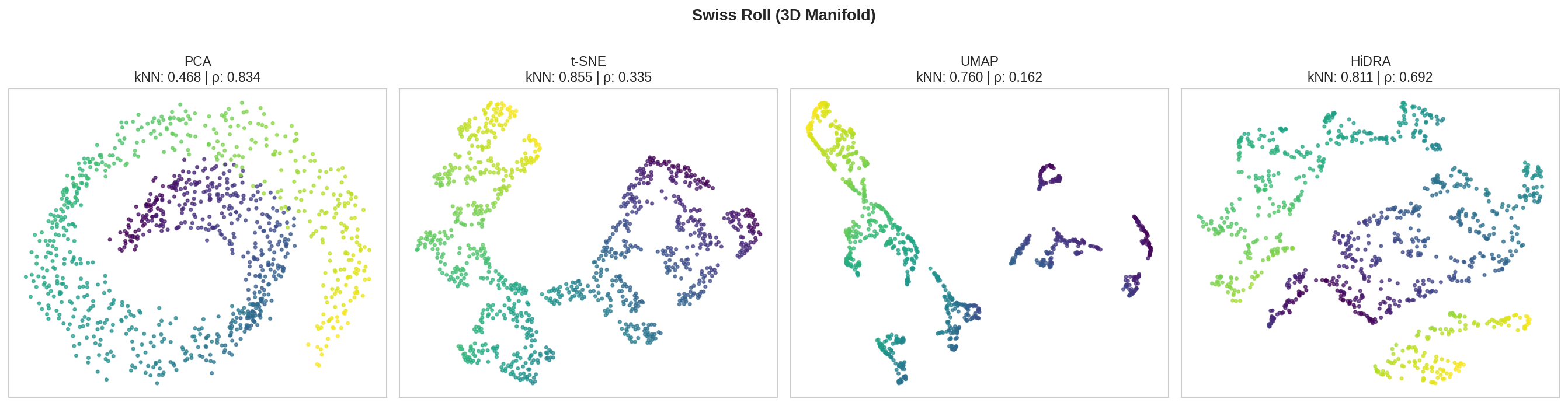
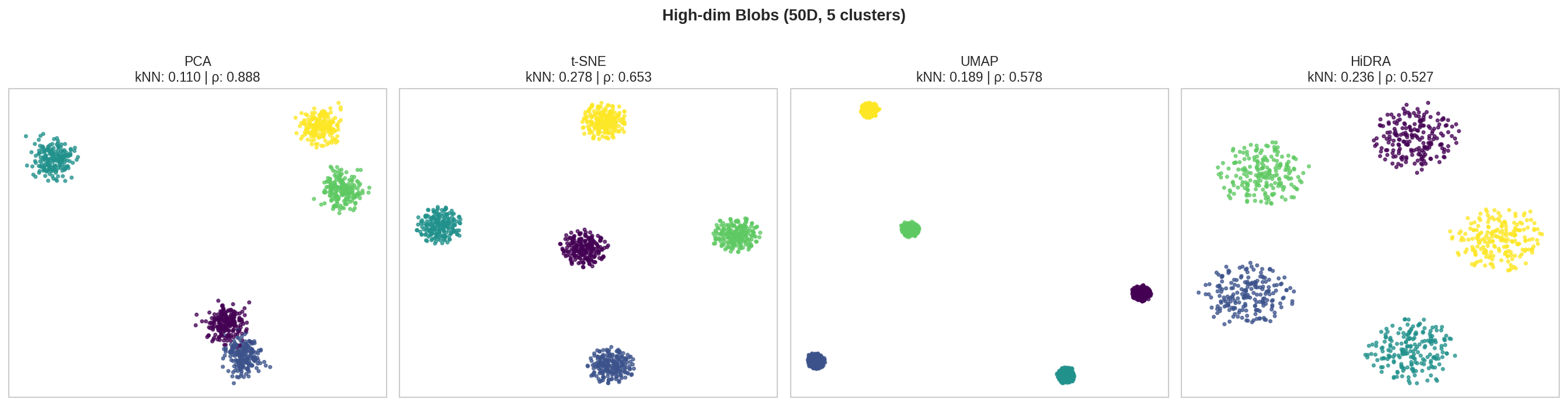
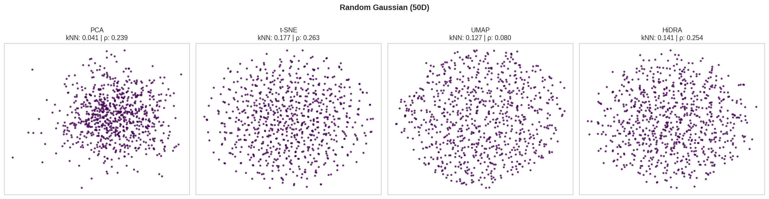
Test datasets: PBMC 3k, Mammoth (3D structure), Swiss Roll, synthetic Gaussians.
Results§
| Dataset | Method | kNN Recall ↑ | Spearman ρ ↑ | Distortion ↓ |
|---|---|---|---|---|
| Swiss Roll | PCA | 0.468 | 0.834 | 229.9 |
| t-SNE | 0.855 | 0.335 | 30.4 | |
| UMAP | 0.760 | 0.162 | 162.1 | |
| HiDRA | 0.811 | 0.692 | 25.2 | |
| S-Curve | PCA | 0.318 | 0.964 | 46.3 |
| t-SNE | 0.833 | 0.898 | 17.3 | |
| UMAP | 0.762 | 0.880 | 91.1 | |
| HiDRA | 0.802 | 0.903 | 29.5 | |
| Blobs 50D | PCA | 0.110 | 0.888 | 89.8 |
| t-SNE | 0.278 | 0.653 | 206.8 | |
| UMAP | 0.189 | 0.578 | 479.5 | |
| HiDRA | 0.236 | 0.527 | 112.8 | |
| Gaussian 50D | PCA | 0.041 | 0.239 | 141.0 |
| t-SNE | 0.177 | 0.263 | 428.2 | |
| UMAP | 0.127 | 0.080 | 83.3 | |
| HiDRA | 0.141 | 0.254 | 100.3 |
- t-SNE: Best kNN (local structure) on all datasets
- PCA: Best Spearman ρ (global structure) on S-Curve and Blobs
- HiDRA: Best balance - beats UMAP on nearly all metrics, competitive with t-SNE on kNN while having much better global structure (ρ) as shown in the high dim structures
- UMAP: Generally underperforms on these benchmarks
Note: These results are from synthetic data from scikit-learn - I have yet to test on real datasets:
from sklearn.datasets import make_swiss_roll
X_swiss, y_swiss = make_swiss_roll(n_samples=1500, noise=0.5, random_state=42)
First iteration did not yield optimal results, as KNN was super low meaning global context was prioritized. I changed from using KNNs to a perplecity-based affinity matrix, PCA instead of geodesic MDS, and changed loss weight cladssifiers to make it just two-phased (exaggeration + dist_w). Instead of the original category losses (near/mid/far), I adapted a KL from t-SNE and optimized using momentum instead of just a gradient descent. Also, computation times were super slow as gradient loops were slow, due to numba I believe. I went back and chnages the distance regularization (the novel aspect of this) which was originally breaking things. Regarding the algorithm, I:
- Fixed gradient computation - The original had a broken kernel normalization that prevented optimization from working
- Cleaned t-SNE-style optimization
- Implemented proportional distance regularization - Added global distance preservation that scaled gradient proportionally to distance+weight and is scale-invariant
I mean PCA has been the gold standard for a while, epecially for population genomics, and it does perform the best here Spearman-wise. I think cotext is important when deciding which to use (PCA vs UMAP), but inter-cluster distances aren't really accurate on UMAPs, which is what HiDRA is trying to solve with multiphase optimization and uncertainity quantification.
The benchmarks show that HiDRA beats standard UMAPs on pretty much everything though which was the goal.